

The current GDP deflator should be 18% higher (in logarithmic form), ie 154.2 instead of 128.2. To see this, consider the tautology:
MV≡PQ
Where Meter it’s money V is the speed, P is the price level, ask is an economic activity.
think V’ is a constant; then:
MV’ = PQ
2019Q4, V stands for M2 It is 1.4245. Get logs (where lowercase letters represent log values).
p = m + v’ – q
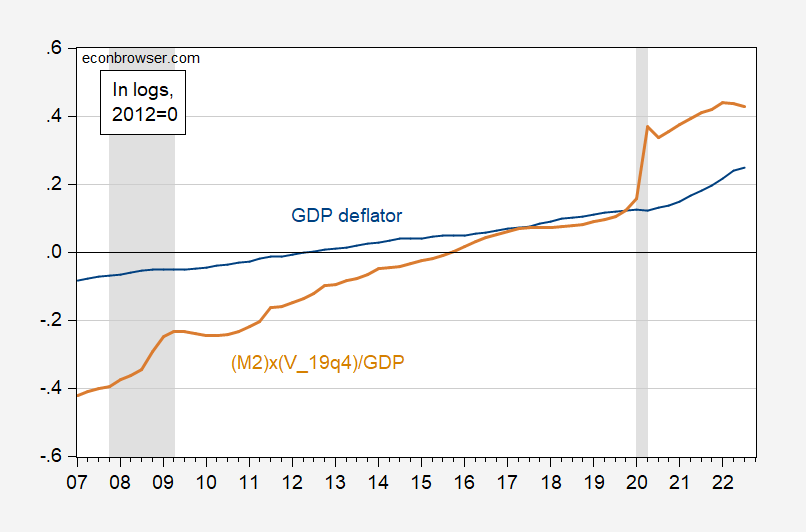
To understand this operation literally, the following figure can be obtained.
figure 1: Log GDP deflator, 2012=0 (blue), log M2 x V’/GDP, where V’ is taken at a constant value of 1.42 (recorded in Q4 2019) (tan). GDP Billion Ch.2012$ SAAR, M2 Billion. Dates of peak-to-trough recessions as defined by NBER are shaded in gray. Federal Reserve, BEA via FRED, NBER, and author’s calculations.
The GDP deflator in Q3 2022 is 25% higher than in 2012, while using the velocity value in Q4 2019, the GDP deflator should be 43% higher (in logarithmic terms) using the price-elastic quantity theory.
In case you were wondering, there is little evidence of velocity stabilization (mean or trend stationarity). The Johansen maximum likelihood method used to test for cointegration shows that there is no evidence that the GDP deflator on the one hand is related to M2 divided by real GDP on the other (brown line in Figure 1) during the period 1960 to the third quarter of 2022. There is a long-term relationship between the brown series).

