

Topic clusters and recommender systems can help SEO experts build scalable Internal Link Architecture.
Internal linking is known to affect user experience and search rankings. This is an area where we want to get right.
In this article, we will use Wikipedia data to build topic clusters and recommender systems with Python and Pandas data analysis tools.
To achieve this, we will use the Scikit-learn library, a free software machine learning library for Python with two main algorithms:
- task force: Term Frequency – Inverse Document Frequency.
- NMF: Nonnegative matrix factorization, is a set of algorithms in multivariate analysis and linear algebra that can be used to analyze multidimensional data.
Specifically, we will:
- Extract all links from Wikipedia articles.
- Read text from Wikipedia articles.
- Create a TF-IDF map.
- Split the query into clusters.
- Build a recommendation system.
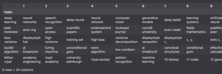
Here’s an example of a topic cluster you’ll be able to build:
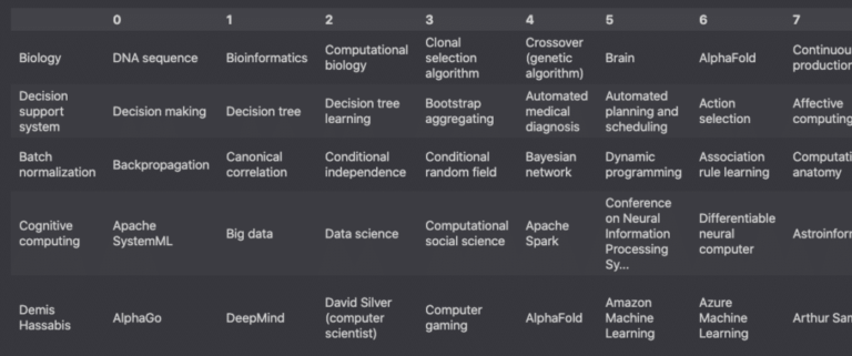
Also, here is an overview of a recommender system that you can recreate.
 Screenshot from Pandas, February 2022
get ready? Let’s start with some definitions and concepts that you want to know.
Difference between topic clusters and recommender systems
Topic clusters and recommender systems can be built in different ways.
In this case, the former is grouped by IDF weight and the latter is grouped by cosine similarity.
In simple SEO terms:
- topic cluster Can help create a schema that all articles link to.
- Recommendation system Can help create a schema that the most relevant pages link to.
What is TF-IDF?
TF-IDF, or Term Frequency – Inverse Document Frequency, is a A number representing the statistical importance of any given word to the entire collection of documents.
TF-IDF is calculated by multiplying the term frequency and the inverse document frequency.
TF-IDF = TF * IDF
- task force: The number of times a word appears in the document / the number of words in the document.
- Israel Defense Forces:log(number of documents/number of documents containing the word).
To illustrate this, let’s consider this situation machine learning As target words:
- Document A contains the target word 10 times out of 100 words.
- In the entire corpus, 30 documents out of 200 also contain target words.
Then, the formula will be:
TF-IDF = (10/100) * log(200/30)
What TF-IDF is not
TF-IDF is nothing new. It’s not something you need to optimize for.
according to John Muellerwhich is an old information retrieval concept that doesn’t deserve SEO attention.
It has nothing to help you outshine your competition.
Still, TF-IDF is useful for SEO.
Understanding how TF-IDF works can provide insight into how computers interpret human language.
Therefore, people can use this understanding to use similar techniques to improve the relevancy of content.
What is non-negative matrix factorization (NMF)?
Non-negative matrix factorization (NMF) is a dimensionality reduction technique commonly used in unsupervised learning, which combines the product of non-negative features into one.
In this article, NMF will be used to define the number of topics we want to group all articles into.
Definition of topic clusters
Topic clusters are groupings of related terms that help you create an architecture where all articles are linked to each other or on the receiving end of internal links.
Definition of Recommendation System
A recommendation system can help create a schema that links the most relevant pages.
Build topic clusters
Topic clusters and recommender systems can be built in different ways.
In this case, topic clusters are grouped by IDF weights and recommender systems are grouped by cosine similarity.
Extract all links from a specific Wikipedia article
Extracting links on Wikipedia pages is done in two steps.
First, choose a specific topic.In this case we use Wikipedia article on machine learning.
Second, use the Wikipedia API to find all internal links to the article.
Here’s how to query the Wikipedia API using the Python requests library.
import requests

main_subject="Machine learning"

url="https://en.wikipedia.org/w/api.php"
params = {
        'action': 'query',
        'format': 'json',
        'generator':'links',
        'titles': main_subject,
        'prop':'pageprops',
        'ppprop':'wikibase_item',
        'gpllimit':1000,
        'redirects':1
        }

r = requests.get(url, params=params)
r_json = r.json()
linked_pages = r_json['query']['pages']

page_titles = [p['title'] for p in linked_pages.values()]
In the end, the result is a list of all pages linked from the initial article.
-
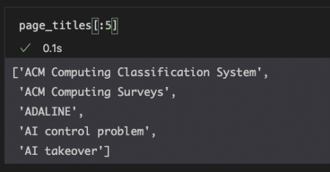 Screenshot from Pandas, February 2022
These links represent each entity used for topic clustering.
Select a subset of articles
For performance purposes, we will only select the top 200 articles (including the main articles on machine learning).
# select first X articles
num_articles = 200
pages = page_titles[:num_articles]

# make sure to keep the main subject on the list
pages += [main_subject]

# make sure there are no duplicates on the list
pages = list(set(pages))
Read text from Wikipedia articles
Now, we need to extract the content of each article to perform the computation for TF-IDF analysis.
To do this, we will fetch the API again for each page stored in the pages variable.
From each response, we will store the text from the page and add it to a list called text_db.
Note that you may need to install the tqdm and lxml packages to use them.
import requests
from lxml import html
from tqdm.notebook import tqdm

text_db = []
for page in tqdm(pages):
    response = requests.get(
            'https://en.wikipedia.org/w/api.php',
            params={
                'action': 'parse',
                'page': page,
                'format': 'json',
                'prop':'text',
                'redirects':''
            }
        ).json()

    raw_html = response['parse']['text']['*']
    document = html.document_fromstring(raw_html)
    text=""
    for p in document.xpath('//p'):
        text += p.text_content()
    text_db.append(text)
print('Done')
This query returns a list where each element represents the text of the corresponding Wikipedia page.
## Print number of articles
print('Number of articles extracted: ', len(text_db))
output:
Number of articles extracted: 201
As we can see, there are 201 articles in total.
This is because we added an article on “machine learning” to the top of the first 200 links on this page.
Also, we can select the first article (index 0) and read the first 300 characters for better understanding.
# read first 300 characters of 1st article
text_db[0][:300]
output:
'nBiology is the scientific study of life.[1][2][3] It is a natural science with a broad scope but has several unifying themes that tie it together as a single, coherent field.[1][2][3] For instance, all organisms are made up of cells that process hereditary information encoded in genes, which can '
Create TF-IDF mapping
In this section, we will rely on pandas and TfidfVectorizer to create a Dataframe containing bigrams (two consecutive words) for each article.
Here we use TfidfVectorizer.
This is equivalent to using a CountVectorizer followed by a TfidfTransformer, which you may see in other tutorials.
Also, we need to remove the “noise”. In the field of natural language processing, words such as “the”, “a”, “I”, “we” are called “stop words”.
In English, Stop words are less relevant For SEO, and overrepresented in the documentation.
So, using nltk, we’ll add a list of English stopwords to the TfidfVectorizer class.
import pandas as pd from sklearn.feature_extraction.text import TfidfVectorizer from nltk.corpus import stopwords
# Create a list of English stopwords stop_words = stopwords.words('english')
# Instantiate the class vec = TfidfVectorizer( stop_words=stop_words, ngram_range=(2,2), # bigrams use_idf=True )
# Train the model and transform the data tf_idf = vec.fit_transform(text_db)
# Create a pandas DataFrame df = pd.DataFrame( tf_idf.toarray(), columns=vec.get_feature_names(), index=pages )
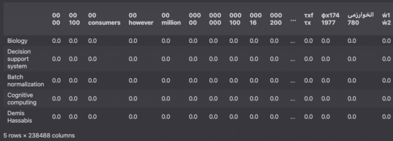
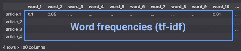
# Show the first lines of the DataFrame df.head()
 Screenshot from Pandas, February 2022
In the above DataFrame:
- Lines are documents.
- Columns are bigrams (two consecutive words).
- These values are term frequencies (tf-idf).
 Screenshot from Pandas, February 2022
Sort IDF vector
Below, we sort the inverse document frequency vector by relevance.
idf_df = pd.DataFrame(
    vec.idf_,
    index=vec.get_feature_names(),
    columns=['idf_weigths']
    )

idf_df.sort_values(by=['idf_weigths']).head(10)
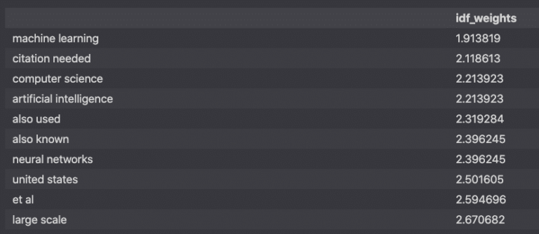 Screenshot from Pandas, February 2022
Specifically, the IDF vector is calculated as the logarithm of the number of articles divided by the number of articles containing each word.
The larger the IDF, the higher the relevance to the article.
The lower the IDF, the more common it is across all articles.
- 1 mention in 1 article = log(1/1) = 0.0
- 1 mention in 2 articles = log(2/1) = 0.69
- 1 mention in 10 articles = log(10/1) = 2.30
- 1 mention in 100 articles = log(100/1) = 4.61
Split queries into clusters using NMF
Using the tf_idf matrix, we split the query into topic clusters.
Each cluster will contain closely related bigrams.
First, we will use NMF to reduce the dimensionality of the matrix to topics.
In short, we will divide the 201 articles into 25 topics.
from sklearn.decomposition import NMF
from sklearn.preprocessing import normalize

# (optional) Disable FutureWarning of Scikit-learn
from warnings import simplefilter
simplefilter(action='ignore', category=FutureWarning)

# select number of topic clusters
n_topics = 25

# Create an NMF instance
nmf = NMF(n_components=n_topics)

# Fit the model to the tf_idf
nmf_features = nmf.fit_transform(tf_idf)

# normalize the features
norm_features = normalize(nmf_features)
We can see that the number of bigrams remains the same, but the articles are grouped into topics.
# Compare processed VS unprocessed dataframes
print('Original df: ', df.shape)
print('NMF Processed df: ', nmf.components_.shape)
Second, for each of the 25 clusters, we will provide query suggestions.
# Create clustered dataframe the NMF clustered df
components = pd.DataFrame(
    nmf.components_,
    columns=[df.columns]
    )

clusters = {}

# Show top 25 queries for each cluster
for i in range(len(components)):
    clusters[i] = []
    loop = dict(components.loc[i,:].nlargest(25)).items()
    for k,v in loop:
        clusters[i].append({'q':k[0],'sim_score': v})
Third, we’ll create a dataframe that displays the recommendations.
# Create dataframe using the clustered dictionary
grouping = pd.DataFrame(clusters).T
grouping['topic'] = grouping[0].apply(lambda x: x['q'])
grouping.drop(0, axis=1, inplace=True)
grouping.set_index('topic', inplace=True)

def show_queries(df):
    for col in df.columns:
        df[col] = df[col].apply(lambda x: x['q'])
    return df

# Only display the query in the dataframe
clustered_queries = show_queries(grouping)
clustered_queries.head()
In the end, the result is a DataFrame showing the 25 topics and the top 25 bigrams for each topic.
Screenshot from Pandas, February 2022Building a recommender system
Instead of building topic clusters, we will now build a recommender system using the same normalized features as in the previous step.
Normalized features are stored in the norm_features variable.
# compute cosine similarities of each cluster
data = {}
# create dataframe
norm_df = pd.DataFrame(norm_features, index=pages)
for page in pages:
    # select page recommendations
    recommendations = norm_df.loc[page,:]

    # Compute cosine similarity
    similarities = norm_df.dot(recommendations)

    data[page] = []
    loop = dict(similarities.nlargest(20)).items()
    for k, v in loop:
        if k != page:
            data[page].append({'q':k,'sim_score': v})
What the above code does is:
- Cycle through each page selected at the beginning.
- Select the appropriate row in the normalized data frame.
- Compute the cosine similarity of all binary queries.
- Select the top 20 queries sorted by similarity score.
After execution, we get a page dictionary with a list of recommendations sorted by similarity score.
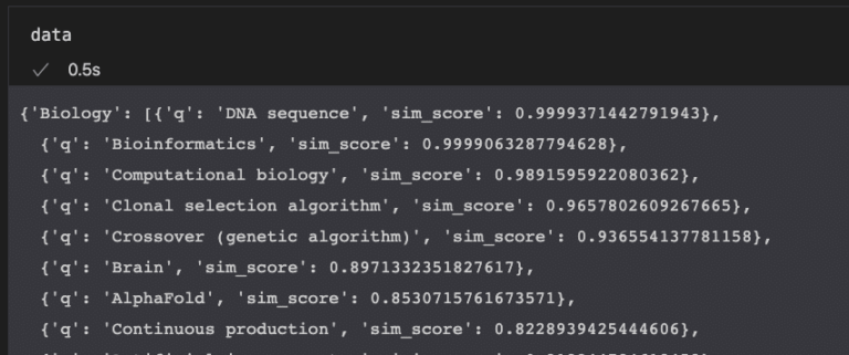 Screenshot from Pandas, February 2022
The next step is to convert the dictionary to a DataFrame.
# convert dictionary to dataframe
recommender = pd.DataFrame(data).T

def show_queries(df):
    for col in df.columns:
        df[col] = df[col].apply(lambda x: x['q'])
    return df

show_queries(recommender).head()
The resulting DataFrame shows the parent query along with the recommended topics sorted in each column.
Screenshot from Pandas, February 2022This is!
We have finished building our own recommender system and topic cluster.
Interesting contributions from the SEO community
I’m a big fan of Daniel Heredia, he also played TF-IDF Find related words using TF IDF, textblob and Python.
Python tutorials can be intimidating.
One article may not be enough.
If so, I encourage you to read Tutorial by Koray Tüberk GÜBÜRwhich exposes a similar way of using TF-IDF.
Billy Bonaros also presented a creative application of TF-IDF in Python, showing How to Create a TF-IDF Keyword Research Tool.
in conclusion
In the end, I hope you’ve learned a logic here that can be adapted to any website.
Understanding how topic clusters and recommendation systems can help improve website architecture is an invaluable skill for any SEO professional looking to expand your work.
Using Python and Scikit-learn, you’ve learned how to build your own – and in the process learned the basics of TF-IDF and non-negative matrix factorization.
More resources:
Featured image: Katerina Reka/Shutterstock
Source link

