

reader Steven Kopitz wrote:
The presentation depends on the data. If you use VMT data, you know that there is a lot of variation, and seasonally adjusted data may not accurately represent seasonal variation. That’s why Menzie’s chart looks like spaghetti.
So how to present it? You can do 3 mma over 3 mma the year before. Still too choppy. You can display annual totals or averages by calendar year, but you’ll miss the turning point. You can make monthly changes, a lamenzi, and get garbage.
But one option is to roll the 12-month average. This removes the whole seasonality issue and provides a nice, smooth graph. On the downside, it may be too late to show an inflection point, and in the current case, the data could be skewed by a rise in VMT in 2021.
So you have to make decisions, and every decision involves some kind of compromise.
I think you’ll agree that Menzie’s diagrams are hard to read, much less understand. I don’t know why he felt the need to do that, since he already had the visuals the last time we discussed the topic.
The only chart in postal This is what was commented on:
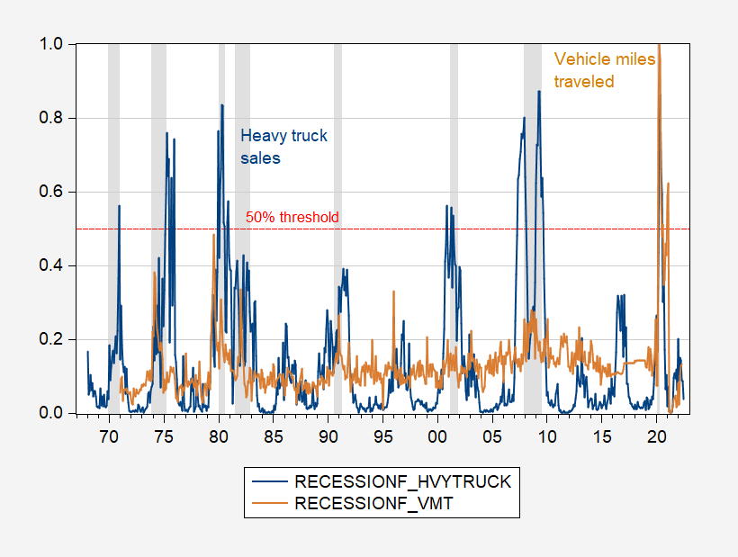
figure 1: Recession probability using 12-month period change in heavy truck sales (blue) and vehicle miles traveled (tan). 50% threshold red dotted line. The NBER uses shades of grey to define the peak and trough dates of the recession. Source: Author’s calculations.
Oddly, Mr. Kopits doesn’t seem to realize—despite the annotations to Figure 1—that this is a graph estimating recession probabilities, not the underlying vehicle mileage (VMT) series (and heavy-duty truck sales).
This is the change in 12-month (logarithmic) vehicle miles traveled, and the change in the 12-month rolling average (2000-2022 period), which Mr. Kopits said he preferred.

figure 2: Change in 12-month vehicle mileage (blue, left scale) and change in 12-month moving average of vehicle mileage in millions (tan, right scale), nsa NBER-defined peak-to-valley decline dates All are shaded in grey. Source: FHA via FRED.
The blue line is the data I used in the probability regression, and the brown line is the one-month change in Mr. Kopits’ preferred measure. The adjusted R2 for one regression to the other is 0.99. In other words, if I were to use Mr. Kopits’ preferred measure, I would get the same implied recession probability.
I tried to be comprehensive in the annotations of the data I provided (especially since then) A reader accuses me of manipulating data), but sometimes I just wonder if it’s worth it because some people can’t read/understand.

