

Confidence interval
reader Steven Kopitz Criticize them:
If historical data is relatively stable compared to future events, confidence intervals, etc. may be useful. So, for example, if we make traffic on the George Washington Bridge and adjust for weather, time of day, day of year, and weekend/holiday, then I think the confidence interval is a useful piece of information. You can make a decision on this basis. …
However, if the data is unstable or not well understood, if the method is new or not well understood, if exceptions to the general rule are not well understood, then the confidence interval may provide a false sense of confidence. For example, if I fail to adjust the GW Bridge numbers for a certain time of day, the confidence interval will be useless. Therefore, if I calculate the average transit time on the bridge, but cross the bridge at 3 am, then I may be too pessimistic about the transit time.
I find that confidence intervals are often used for political purposes to predict methodological certainty of exaggerated situations. Sometimes it is material. Hurricane Maria in PR is a case study.
Readers will remember that Mr. Kopits provided a series of estimates for Hurricane Maria, which later proved to be too low.exist 5/31/2018 He wrote:
I predict that the total number of excess deaths within a year (for example, by October 1, 2018) may reach 200-400.
He then increased his estimate on June 4 to 1,400 in December 2017 (see this postal For discussion). You can see the various estimates listed by Sandberg et al. (2019) here.
To summarize graphically:
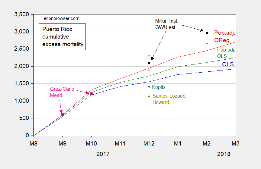
figure 1: The cumulative number of excess deaths since September 2017, based on the simple time dummy variable OLS model (blue), the population-adjusted OLS model (green), and the population-adjusted quantile regression model (red), Milken Research Estimated value (black square) and 95% confidence interval (grey +), Santos-Lozada, Howard letter (yellow-green triangle), Cruz-Cano and Mead (pink square), Kopits (blue-green triangle). Not above picture: Kopits estimate 300-400 in October 2018. Source: author’s calculations, Milken Institute (2018), Santos Losada and Howard (2018), Cruz-Kano and Mead (2019), and Kopits (2018).
For a long-term study where Mr. Kopits failed to understand what the confidence interval is, please refer to this postal.
So, my point-confidence interval is very useful. Even if they are wide (in this case, they will tell you to pay attention to the deterministic alarm sound). Of course they defeated the “pull it out of a gang” method.Since Mr. Kopits is unlikely to believe me, I will Pay attention to David Romer’s praise of the confidence interval.
The last point about the confidence interval: Regarding the question of conditional changes (I am not sure what “unstable data” is), there are some ways to explain the time change of standard errors. The simplest idea (I teach my undergraduates!) is to do a rolling regression. Consider regression:
Δp$import = α + βΔsecond$ +you
This can be estimated by rolling the window, in this case 24 months. I use BLS to measure commodity import prices for the variable on the left, and use the (nominal) broad trade-weighted dollar exchange rate for the right (both recorded, first-order difference). For the complete sample:
Δp$import = 0.002 + 0.44Δsecond$ +you
Adj-R2 = 0.22, SER = 0.011, Nobs = 314. Black body Means significant at 5% msl, using HAC robust standard error (Newey-West).
The beta coefficient estimate and the standard error of +/- 1.96 are as follows:
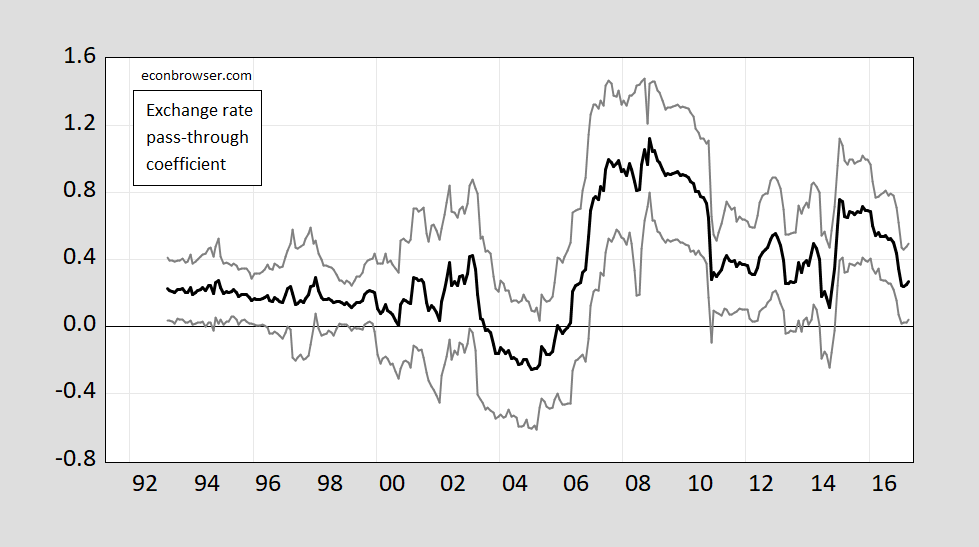
figure 2: The exchange rate passes a rolling regression coefficient, a 24-month window (black), and a standard error of +/- 1.96 (grey line). Source: Author’s calculations.
Log
About my long beach port traffic time series chart, Steven Kopitz Wrote:
Why do you even think of using logarithms to represent it? It’s totally deceptive. Directly on the picture.
I actually think that it is deceptive to map things horizontally when people are interested in growth rates. Consider the PCE deflator. If you plot by level, the price level seems to have been increasing at a constant rate from 1985 to 2020. The straight line in the logarithmic scale with e as the base represents a constant growth rate).
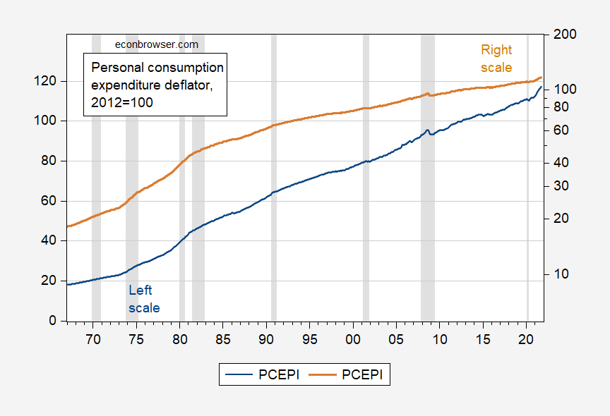
figure 2: Personal consumption expenditure deflator (blue, left scale), personal consumption expenditure deflator (brown, right log scale). NBER-defined recession dates are shaded gray from peak to trough. Source: BEA, NBER.
For more information on counter-log utterances, please refer to this postal.
Question for everyone: Do they still teach logarithms and powers in high school?

