

Two methods of calculating how prices move before and during a pandemic, combining the concepts of stochastic and deterministic trends (e.g., postal, Stock and Watson, JEP, 1988).
In short, look at the difference in inflation (which I think is natural) or the trend in log relative prices (follow this up postal).
figure 1: Monthly core inflation differential between the US and the Eurozone (black), calculated using the log-first differential. The cyan line is the (annualized) 2018-2020M1 average difference; the red line is the (annualized) average difference 2020M02-2022M03. The authors seasonally adjusted core HICP for the euro area using geometric census X-12. The NBER uses shades of grey to define the peak and trough dates of the recession. Source: BLS, Eurostat via FRED, NBER and author’s calculations.
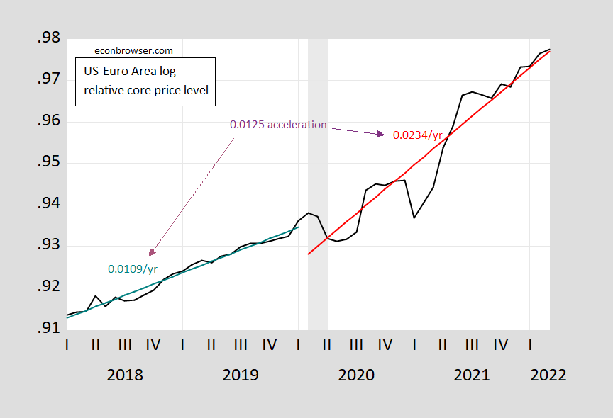
figure 2: Seasonally adjusted log ratio of US core CPI to Eurozone HICP core (black). Use the fitted values of the estimated equation (cyan, red). The blue-green line is the (annualized) trend difference 2018-2020M1; the red line is the (annualized) trend difference 2020M02-2022M03. The authors seasonally adjusted core HICP for the euro area using geometric census X-12. The NBER uses shades of grey to define the peak and trough dates of the recession. Source: BLS, Eurostat via FRED, NBER and author’s calculations.
Using the (annualized) inflation differential approach, inflation accelerated by 0.7 percentage points, but the coefficient was not estimated precisely (mechanically, because of the high variance of inflation differentials during the pandemic). Using the log-ratio trend growth, the acceleration in price level growth was 1.25 percentage points and was statistically significant, even with Newey-West standard errors (t-stat 6.64).
What is the “correct” way? The first is more suitable for regression-based diffs-in-diffs methods (I looked at how the inflation difference changes before and after). The second is how people usually figure out how trends are changing if one isn’t particularly worried about random trends (you probably won’t go beyond such a short sample).
In any case, the regression of the inflation differential on constant and epidemic dummies has an R2 0.01, DW = 1.73. Regression of Logarithmic Alignment Constant, Time Trend, Popularity Dummy, Interaction of Popularity Dummy and Time Trend with R2 is 0.96, DW = 0.71. These regression results are characterized by spurious correlations, i.e. R2 > DW, so I’m reluctant to overinterpret the finding of statistical significance using traditional estimates of standard errors, the mean.
Inflation differential rejects the unit root ADF and Elliot-Rothenberg-Stock DF-GLS null hypothesis, but fails to reject the KPSS trend stationary null hypothesis; log relative core price fails to reject the ADF and DF-GLS null but rejects the KPSS trend stationary null hypothesis .
The trend method can be verified by testing whether the unit root null is rejected allowing the structure to break the test. I implement Perron’s (1989) unit root/breakpoint test using innovative outliers (allowing for constants and trends). In this case, the program rejects the unit root in favor of trend stationarity and breaks in 2021M03. The re-estimation allows the relative price regression equation to break out in 2021M03 to yield an implied acceleration of 1.6 percentage points to the relative trend.

image 3: Seasonally adjusted log ratio of US core CPI to Eurozone HICP core (black). Fitted values (blue, dark red) using the estimated equation. The blue line is the (annualized) trend difference 2018-2021M2; the dark red line is the (annualized) trend difference 2021M03-2022M03. The authors seasonally adjusted core HICP for the euro area using geometric census X-12. The NBER uses shades of grey to define the peak and trough dates of the recession. Source: BLS, Eurostat via FRED, NBER and author’s calculations.

