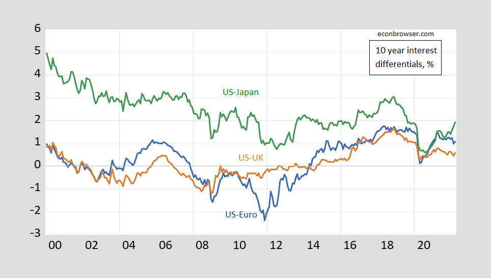


Some key spreads as of March:
figure 1: Ten-year government bond yield spreads US-Euro area (blue), US-UK (brown), US-Japan (green), expressed as a percentage. Source: OECD MEI from FRED, Treasury (US) and author’s calculations.
As we move away from the zero lower bound (again) and we see faster inflation, I think it will be interesting to see what links may exist between long-term interest rates. In particular, will long-term interest rates be in line with the expected rate of depreciation?
The answer to this question is imprecise because we don’t directly observe market expectations; on a 10-year scale, we don’t actually have much survey-based expectations data (this is in contrast to year-long short-term data such as Busier et al. (2022)).However, we can observe how subsequent afterwards The exchange rate moves with the spread – until the first quarter of 2012. The past tells us what to expect.
exist Chin and Meredith (1998), we document that the spread is positively related to ex post depreciation in the long run. The panel regression coefficients have the following pattern:
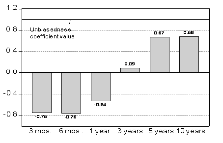
figure 2: Panel betas for different time periods. Note: Up to 12 months, panel estimates 6 currencies against USD, Euro deposit rate, 1980Q1-2000Q4; 3-year result is zero coupon yield, 1976Q1-1999Q2; 5-year and 10-year, yield to maturity is not Change, 1980Q1-2000Q4 and 1983Q1-2000Q4 (last observations correspond to exchange rate data). source: Chin (2006).
I updated these results four years ago postal (Earlier, in Chinn and Quayyum (2013). We can do this by using Return of Fama,which is. :
(1) st+k -sTon = α + β(A generationTonK-A generationTonk*) + et+k
Where s is the logarithmic exchange rate defined as the domestic currency unit per foreign currency unit (e.g., US dollars per pound for Americans); A generationTonK is the remaining interest rate to maturity Kand * means a foreign country (for example, the United Kingdom); and e is a wrong term.
Coefficient test b Not Different from Unity is a Test of “Unbiasedness” – The Joint Null Hypothesis of Interest Parity Not Found and Average expectations are correct (or all information held by rational expectations).
Regressing the US-UK quarterly data (period end) yields:
st+k -sTon = -0.002 + 0.554(A generationTonK-A generationTonk*) + et+k
adjust -R2=0.21, SER=0.018, DW=0.018, Nobs=157, sample 1983Q1-2022Q1. bold Indicates significantly different from the unity value of the HAC robust standard error using 5% msl.
In this case, for quarterly data, k=40. This regression result summarizes the relationship in this scatterplot:
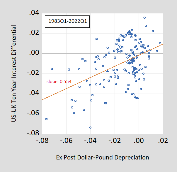
image 3: The 10-year USD/GBP ex post depreciation annualized to the 10-year US-UK 10-year spread lags 10 years.
For the US-Euro area:
st+k -sTon = 0.003 + 0.592(A generationTonK-A generationTonk*) + et+k
adjust -R2=0.05, SER=0.024, DW=0.011, Nobs=53, sample 2009Q1-2022Q1. bold Indicates significantly different from the unity value of the HAC robust standard error using 5% msl.
USA – Japan:
st+k -sTon = 0.015 + 0.323(A generationTonK-A generationTonk*) + et+k
adjust -R2=0.02, SER=0.032, DW=0.058, Nobs=157, sample 1983Q1-2022Q1. bold Represents significantly different from unity using HAC robust standard errors.
In previous studies, Japan’s coefficient was particularly low and striking. One explanation is the lack of capital account liberalization early in the period. Starting to examine the interest rate data for the first quarter of 1982 (hence looking at the 10-year exchange rate changes from the first quarter of 1992), we get:
st+k -sTon = -0.033 + 1.699(A generationTonK-A generationTonk*) + et+k
Adj-R2=0.28, SER=0.028, DW=0.161, Nobs=121, samples 1992Q1-2022Q1. bold Indicates that the robust standard error using HAC at 5% msl is significantly different from a unit value (slope) or zero (constant).
Therefore, the coefficients of the long-term Fama regression are usually positive (still), and zero values of the unit slope coefficients are not rejected in some cases. Having said that, it is unclear whether this correlation largely guides the adjusted R2is too low.