

Amid the debate over whether the agency survey nonfarm payrolls data series has grossly overstated recent employment, especially in the second quarter, one reader Asked indignantly: “So you’re saying the Philly Fed screwed up its analysis and we should ignore its work? Is that your take?”. Short answer to the first question: no. Short answer to your second question: see below.
I take the lead Zhou Lian A method of interpolation/extrapolation by related series and exploiting the close relationship between the overall movement of the total employment series covered in the Quarterly Census of Employment and Wages (QCEW) and the non-farm employment series. Specifically, I follow this procedure:
- Estimated relationship between log NFP employment and log total covered employment for 2001-2019.
- Use this relationship to predict in-sample and out-of-sample NFP employment
- Verify that NFP employment is well predicted in the out-of-sample period.
- Explanation
In order for people with statistical difficulties to understand the program (eg, People who don’t know what a confidence interval is), showing what I did in the step.
- estimate
I collected total employment data covered by NFP (FRED series PAYNSA) and QCEW for the period 2001-2022 (QCEW data starts from 2000M12). QCEW data come from the census and therefore should not be affected by sampling error (QCEW data are used to benchmark updates to estimates based on the CES survey). Unfortunately, total employment covered by the QCEW is not reported on a seasonally adjusted basis. Therefore, I estimated the relationship between the non-seasonally adjusted series, expressed logarithmically. These data are shown in Figure 1.
figure 1: Nonfarm payrolls (blue), total employment covered (tan), 000, not seasonally adjusted.Non-agricultural data series is FRED series PAYNSA; total coverage series is BLS series ENUUS00010010. Dates of peak-to-trough recessions as defined by NBER are shaded in gray. Source: U.S. Bureau of Labor Statistics.
Note that the correlation is very high. Running the regression (to 2019), the statistical fit is very good with an adjusted R2 of 0.997.
Note that the constants are very small and the coefficients are close to (but significantly different from) 1. Still, we’re interested in predictions, so it doesn’t really matter. To prevent spurious correlations, I test for cointegration using Johansen’s maximum likelihood method. I reject null values at 10% for zero cointegrated vectors (cointegrated vectors are constant, no trend).
Why not estimate the entire sample until 2022? This produces a fit like:
However, tests using recursive residuals to assess structural breaks show a break at 2020M07, supporting the use of samples that ended before the pandemic started; as shown in Figure 2.
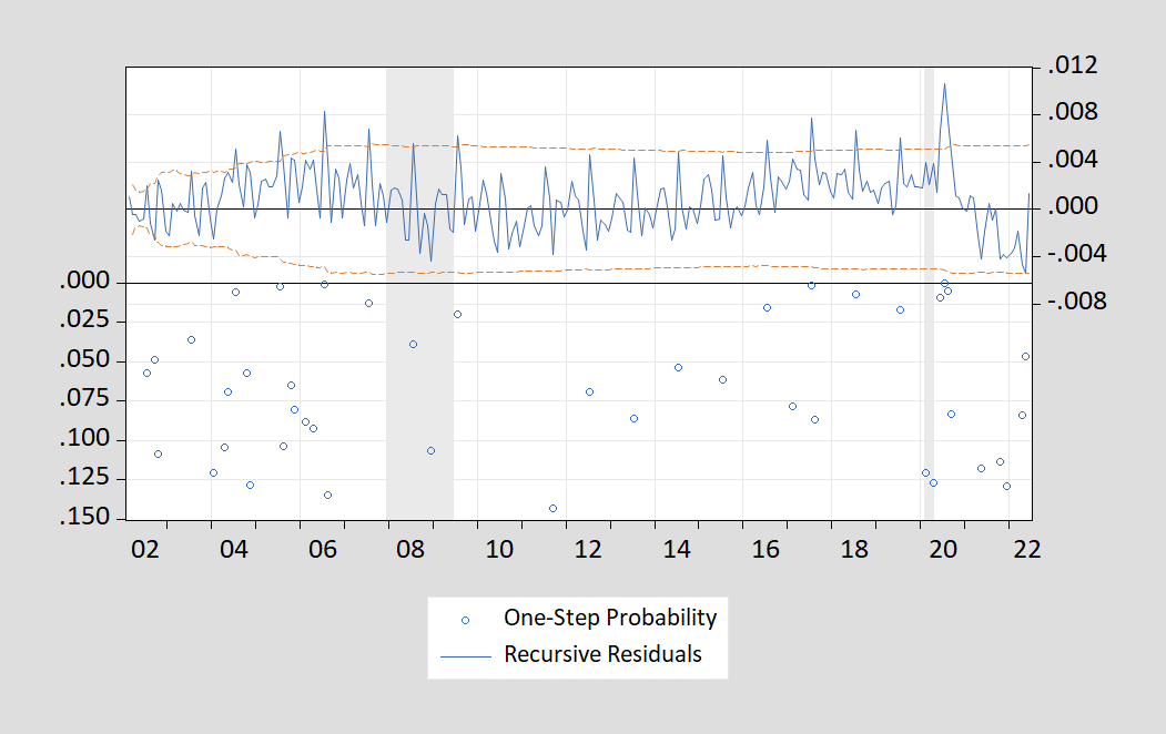
figure 2: Recursive residuals from regression of log PAYNSA on log total covered QCEW employment. P-values on the LHS scale.
- prophecy
I use the equation estimated for 2001-19 to forecast non-seasonally adjusted NFP (PAYNSA). as shown in picture 2.
The fit tracks the reported series well. This is expected since the BLS series was benchmarked using QCEW data.
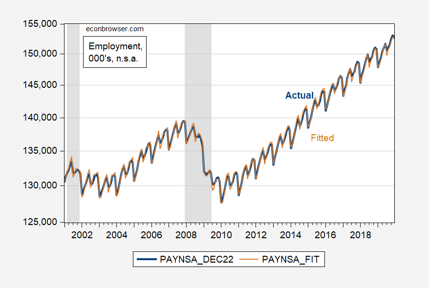
image 3: Reported nonfarm payrolls, unadjusted for seasonality (blue), fitted (tan). Dates of peak-to-trough recessions as defined by NBER are shaded in gray. The shade is light green during the sample period. Sources: BLS, NBER, author’s calculations.
- not suitable for sample
The equations used to fit the model were estimated for the period up to 2019M12. This means 2020-2022M06 is outside the sample period that can be assessed (since QCEW data ends in 2022M06). These predictions are shown in Figure 4. Green indicates the in-sample period.

Figure 4: Reported nonfarm payrolls, unadjusted for seasonality (blue), fitted (tan), 95% prediction interval (gray line). Dates of peak-to-trough recessions as defined by NBER are shaded in gray. The shade is light green during the sample period. Sources: BLS, NBER, author’s calculations.
During the pandemic lockdown, the mean error is 50k (remember that NFP employment is currently around 253m), the maximum is 1.9m, the minimum is -866k, and the standard deviation is 582k.
- impact on the debate
Interestingly, the model tends to underestimate reported employment by a large margin. In other words, if the historical correlation holds, the implied NFP should actually be higher than reported. Nonfarm payrolls should have risen by 291K in March; NFP was reported 155K higher than expected in June, so we don’t have some evidence of overestimation until June. While the reported NFP was higher than expected, the number was well below the Philadelphia Fed’s forecast of nearly 1 million.
These are not seasonally adjusted series. To convert my forecasts to values compatible with the commonly referenced seasonally adjusted series (PAYEMS), I added the seasonal component of the BLS (PAYEMS-PAYNSA) estimate to the forecasts shown in Figure 4. I show this implied sequence and the actual in Figure 5.
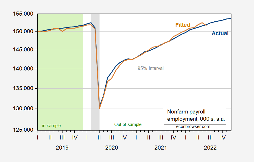
Figure 5: Reported nonfarm payrolls, both seasonally adjusted (blue) and fitted (tan), are 000, with SA NBER defined recession peak-to-trough dates in gray. The shade is light green during the sample period. Sources: BLS, NBER, author’s calculations.
I show recent details, as well as the BLS research series adjusting the civilian employment (household survey) series to the NFP concept (green line), and the Philadelphia Fed adjusting the QCEW data to fit the NFP (red squares), in Figure 6.

Figure 5: Reported Nonfarm Payrolls, Seasonally Adjusted (Blue), Fitted (Tan), BLS Research Series Civil Employment Adjusted to NFP Concept (Green) and Philly Fed Series (Red Squares), All 000, SA NBER Definition The peak and valley recession dates are grayed out. Sources: U.S. Bureau of Labor Statistics, Federal Reserve Bank of Philadelphia, and authors’ calculations.
My nonfarm payrolls for March line up pretty well with the Bureau of Labor Statistics series, both nsa and sa (where I use BLS seasonal adjustment). My first observation was to notice that this is a quick and dirty method. It is not a comprehensive defense of the benchmark unrevised series. Of course, there are reasons why building series go off track. In their “overall” assessment, House and Pugliese/Wells Fargo Highlights the fact that the birth/death model may have introduced too many new companies being created, pushing up non-farm payrolls. However, I’m using QCEW for tracking, which is immune to such estimation errors.
My second observation is that the fact that the Philly Fed series suggests that NFP is much lower does not mean that one way or the other is wrong. This could mean that the seasonal adjustment process is distorting the results (either on the BLS side, or on the Philly Fed side, recall how they switch between geometric and additive errors), or that the Philly Fed is coordinating the states/departments The way the data are QCEW and business surveys introduces measurement errors. In this case, time will tell. The civilian employment series is always lower than the official BLS series.Perhaps the household series provide a better employment signal than the establishment and quarterly censuses of employment and wages (remember this is a census), but this is a little hard to understand for me.

