

Suppose you want to measure the relationship between multiple variables. One of the simplest methods is to use linear regression (for example, the ordinary least squares method). However, this method assumes that the relationship between all variables is linear. One can also use a generalized linear model (GLM) to transform the variables, but the relationship between the results and the transformed variables is – you guessed it – linear. What if you want to model the following relationship:
In this data, both variables are normally distributed with a mean of 0 and a standard deviation of 1. Furthermore, this relationship is largely comonotonic (i.e., as the x variable increases, so does y). However, this correlation is not constant. These variables are strongly correlated for smaller values but weakly correlated for larger values.
Does this relationship really exist in the real world? Of course it is. In financial markets, the returns of two different stocks may show a weak positive correlation when stocks rise or rise; however, during financial crises (e.g., COVID-19, dot-com bubble, mortgage crisis), all stocks fall, So the correlation will be very strong. Therefore, it is very useful to make the dependence of different variables change with the value of a given variable.
How to model this type of dependency? A Kiran Karra’s amazing video series Explain how to use copulas to estimate these more complex relationships. To a large extent, copulas are constructed using Sklar’s theorem.
Sklar’s theorem states that any multivariate joint allocation Can be written as a single variable marginal distribution Dependent structural connections between functions and description variables.
https://en.wikipedia.org/wiki/Copula_(Probability Theory)
Copulas are popular in high-dimensional statistical applications because they allow one to easily model and estimate the distribution of random vectors by estimating marginals and copulas separately.
Each variable of interest is converted into a uniformly distributed variable ranging from 0 to 1.In the Karra movie, the variable of interest is X and y Uniform distribution is you and v.According to Sklar’s theorem, you can convert these uniform distributions to any distribution of interest using the inverse cumulative density function, the function F-Inverse and G– respectively inverse.
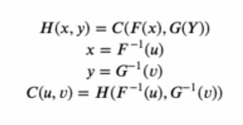
Essentially, the 0 to 1 variables (u,v) are used to rank numerical values (i.e. percentiles). Therefore, if u=0.1, the 10th percentile value is given; if u=0.25, the 25th percentile value is given.What the inverse CDF function does is, if you say u=0.25, the inverse CDF function will give you the expected value X At the 25th percentile. In short, while the math looks complicated, we can really only use marginal distributions based on 0,1 ordered values. More information on the math behind connections is below.
The next question is, how do we estimate copula using data? To do this, there are two key steps. First, you need to determine which copula to use, and second, you must find the copula parameters that best suit the data. Copula essentially aims to find the underlying dependence structure (where dependence is based on levels) as well as the marginal distribution of individual variables.
To do this, you first convert the variable of interest into a ranking (basically, change x,y Enter UV rays in the example above). Below is a simple example where continuous variables are converted into ranked variables. To increase the u,v variables, simply divide by the maximum rank + 1 to ensure that the value is strictly between 0 and 1.
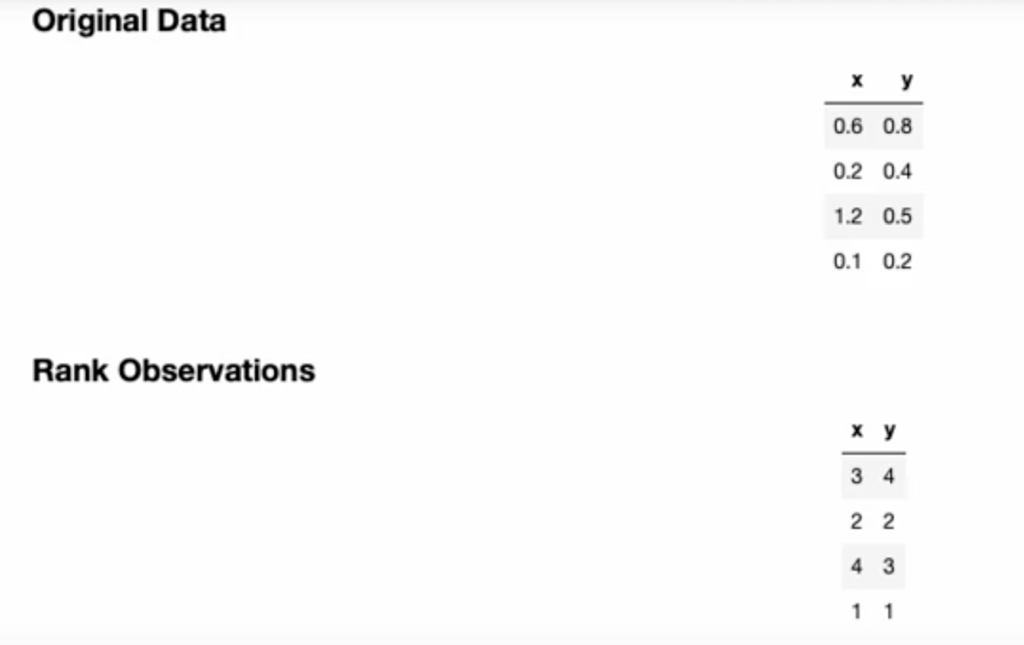
Once we have our rankings, we can use Kendall’s Tau (aka Kendall rank correlation coefficient). Why do we use Kendall’s Tau instead of regular correlation? The reason is that Kendall’s Tau measures the relationship between grades. Therefore, Kendall’s Tau is the same for the original and sorted data (or conversely, for any inverse CDF for marginal values conditioned on the relationship between u and v). In contrast, the Pearson correlation between raw and ranked data may differ.
One can then choose a copula form. Common connections include Gaussian connection, Clayton connection, Gumbel connection and Frank connection.
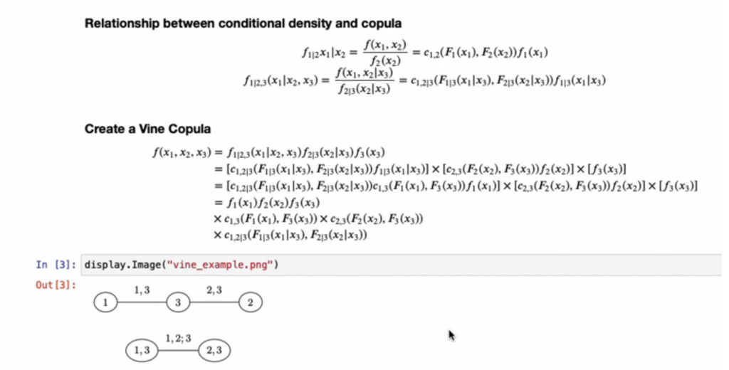
The example above is for two variables, but one of the advantages of the copula is that it can be used with multiple variables. Computing the joint probability distribution over a large number of variables is often complex. Therefore, one way to make statistical inferences over multiple variables is to use a vine copula. Vine copula dependence chain (or vine) or conditional marginal distribution.In short, an estimate
For example, in the following 3-variable example, estimate the joint distribution of variables 1 and 3; the joint distribution of variables 2 and 3, and then estimate variable 1 conditional on variable 3 and variable 2 conditional on variable 3. Distribution. While this seems complicated, essentially, we are doing a series of pairwise joint distributions, rather than trying to estimate a joint distribution based on 3 (or more) variables simultaneously.
The following video introduces vine copulas and how to use them to estimate relationships between more than 2 variables using copulas.
For more details I recommend watching Full range of videos.

